Comparison Solver

The Comparison solver analyses the relationship between two input sources, Input A and Input B. It analyzes whether Input A is; above Input B by a certain distance, below Input B by a certain distance, or near Input B within a certain distance.
Tip: If you want to compare an indicator to two fixed numeric values, then use the Threshold solver.
BloodHound v2
Properties tab
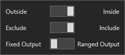
This section provides quick access to commonly used output modifiers.
Please note: The buttons only modify the individual instance of the selected node(s) on a Logic Board. Thus, the buttons are only visible when a node is selected on the Logic Board. The buttons are not available when a solver is selected in the Solvers panel, because the original solver's output can not be globally modified.
This behavior is consistent with adding a function node afterwards, so that the original solver's output remains unmodified elsewhere in the system. It is similar to having an SMA(50) on several charts. Changing the plot color on one chart does not modify the plot color on the other charts.
Global Properties
Global Properties
Behavior
Input A
This is the first input data to be evaluated against Input B. Use the Type drop-down menu to select the data type.
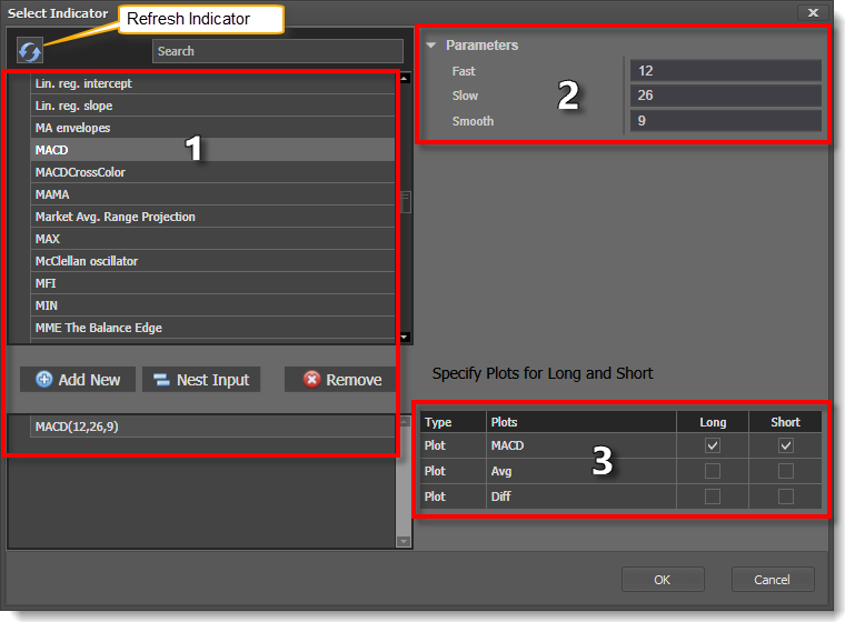
The menu will change based on which data type is selected. Click on Type to see the various data types available and the corresponding documentation.
The Input section determines the data type to be evaluated. Use the 'Type' menu to select the data type. See below for detailed information on each data type.
Type: Fixed Value
Type: Price
This option allows price data to be used in the solver. The price data can be shaped/manipulated by the various settings before it is used by the solver.
Custom Prices
SharkIndicators has custom system development prices that are very useful in reducing the number of solvers, and simplifying system logic, when evaluating the open and close (body) prices.
Body Top: Regardless of the bar direction, this returns the upper price of the candlestick body. Either the close or open price. Whichever is on top. e.g. For an up bar, the Body Top equals the close price.
Body Median: This returns the median price of the candlestick body. The formula is (Close + Open) ÷ 2.
Body Bottom: Regardless of the bar direction, this returns the lower price of the candlestick body. Either the close or open price. Whichever is the bottom. e.g. For an up bar, the Body Bottom equals the open price.
Type: Volume
Volume will feed the current bar volume into the solver.
To evaluate the volume from a few bars back, use Indicator Value. Then select the VOL indicator, and use the Displacement setting.
Type: Indicator Value
Type: Swing Point Prices
Swing Point Prices uses the Swing Highs & Lows indicator plots for input price data. This is useful when you need to access the lowest low or highest high prices from the latest swing point.
You can add the bundled indicator Swing Highs & Lows to the chart to help you visualize the price data the solver is using.
Type: Linear Regression Channel
Selecting Regression Channel allows you to use the Regression Channel Upper, Middle, or Lower line as input to the solver. This may be useful if you need to compare an indicator or price to one of the Regression Channel lines. Select which channel lines to use as input for the long and short evaluations separately, with a choice of the Upper Channel Line, Middle Channel Line, or Lower Channel Line.
Note: Using the Regression Channel for slope related solvers (Slope, Change in Slope, and Inflection solvers) do not have a channel selection since the slope for all channel lines are always the same. As you may expect, the slope of the channel line is what is evaluated, which is the same as using the 'Lin. reg. slope' indicator for the input.
Input B
This is the second input data to be evaluated against Input A. For documentation scroll up to section Input A.
Use the Type drop-down menu to select the data type. The menu will change based on which data type is selected.
Output
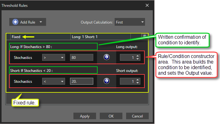
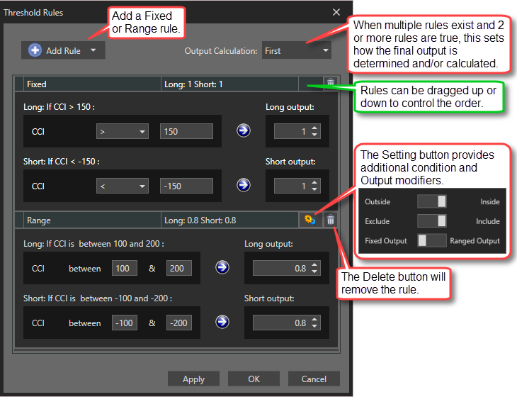
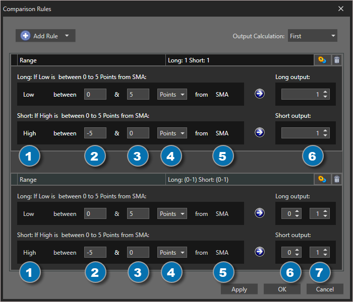
 Settings window: This applies to the Range rule. It provides more detailed control over the values being evaluated.
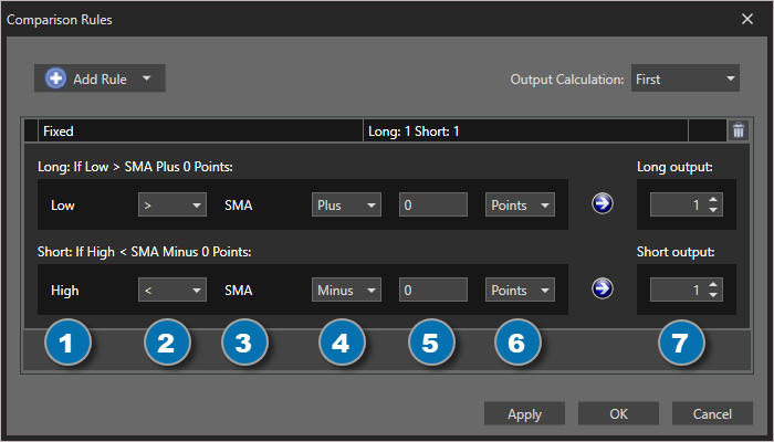

Options tab
This section is used to modify the node's final output value. It is only useful for designing fuzzy logic systems, or a fuzzy logic section of a system.
Please note: The Weight controls only modify the individual instance of the selected node(s) on a Logic Board. Thus, the Weight controls are only visible when a node is selected on the Logic Board. The controls are not available when a solver is selected in the Solvers panel, because the original solver's output can not be globally modified.
This behavior is different than BloodHound 1.0. In BH 1.0, the Weight controls modified the nodes output globally (every instance). This change in BH 2.0 adds more system design granularity.
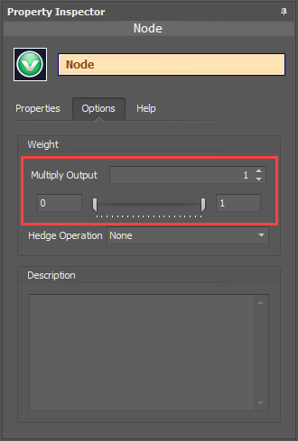 Multiply Output: This takes the internal values (the Long and Short values determined via the Properties tab » Output Rules section) and multiplies them by this value.
Note: The final output will not exceed a value of 1, as described in the Slider control below.
Slider control: The slider constrains the final output to a value of 0 to 1. The left side of the slider sets a minimum value that is output regardless if the solver condition is true or not. The right side sets a maximum value that is output. The output is capped.
e.g. Three indicator conditions are being checked, and thus three solvers are created. Only two out of the three indicator conditions are needed. An Additive logic node is used to add the solver's outputs together. Just two out of the three solvers need to add up to a value of 1. Therefore, the right slider (max output value) for all three solvers is set to 0.5. When two indicator/solver conditions are found, thus the outputs = 0.5, then the calculation, in the Additive node, is 0.5 + 0.5 + 0 = 1. A value of 1 means the two out of three condition is true.
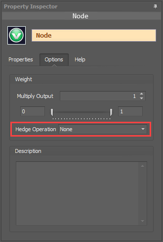 Hedge Operation: This applies a mathematical formula to the internal value.
None: No modification is applied.
Very (square output): A squaring formula is applied. Output = value^² .
Somewhat (square root output): A square root formula is applied. Output = √value .
Description
Description
This text area provides a place to write a full description of what the node is doing, used for, or what ever you want.
Note: The Description is global to all instances of the node. It is not applied individually to each instance as the Weight controls are.
Help tab
This tab displays the documentation page (from this web site) of the selected node.
Please note: NinjaTrader v8.0.26.0 or newer is required for the built in web viewer to work, and thus the documentation to be displayed.
Video Tutorial
Example: Entire Bar is Above/Below SMA20 Trend Filter (3 minutes)
Examples
Example 1A: A Basic Trending State
(Bar Above / Below SMA)
This example identify when the entire bar is above or below the SMA 14. A long output occurs when the bar is above, and a short when the bar is below.
Input A & B Settings:
Note that the Low price is used for the Long output calculation. That is because for the entire bar to be above the SMA, the bottom or lowest price must be above the SMA, or else the bar would be touching the SMA.
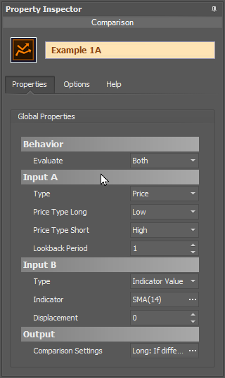
- Set Input A » Type to Price.
- Set the 'Price Type Long' to the Low price.
- Set the 'Price Type Short' to the High price.
- Leave Input B as the SMA 14.
Rules window Settings:
No changes are needed to the Rules window.
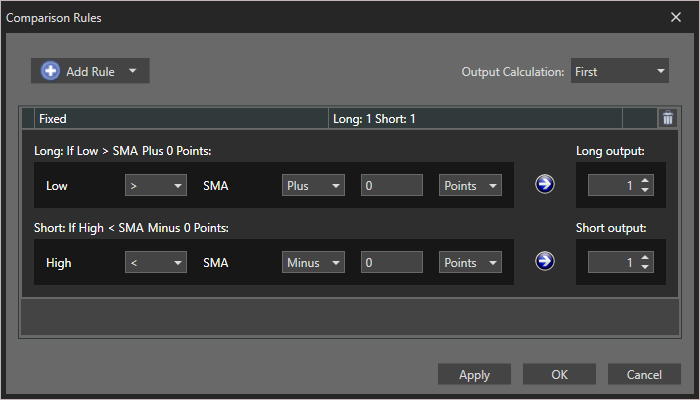
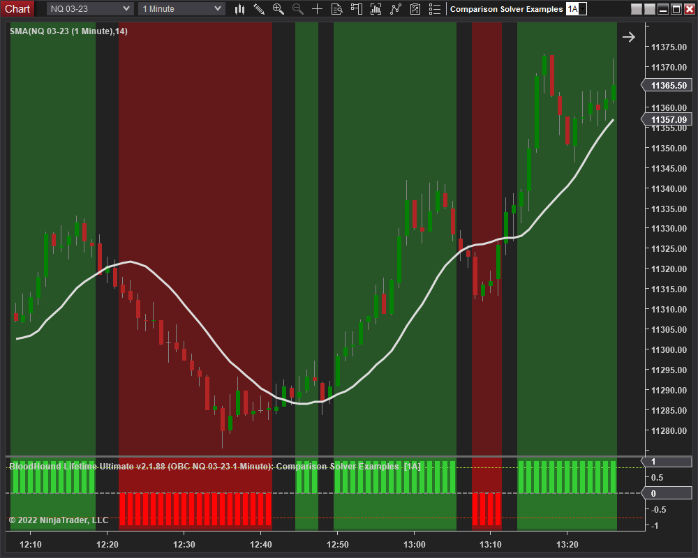
The chart below shows a Long output when the Low price is above the SMA 14, or a Short output when the High price is below the SMA 14. If there is no output, the bar is touching the SMA.
Example 1B: Setting a Minimum Separation Distance
This example identify when the SMA 14 is 5pts or more, above or below the SMA 50. A long output occurs when the SMA 14 is 5pts or more above the SMA 50, and and vise versa for a short output. There is no output when the SMA's are within 5pts of each other.
Input A & B Settings:
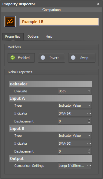
- Input A is unchanged as the SMA 14.
- Input B is adjusted to the SMA 50.
Rules window Settings:
Open the Rules window by clicking the ellipses button in section Output » Comparison Settings.
- Note that setting ➄ is set to 5.
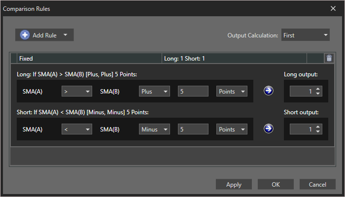
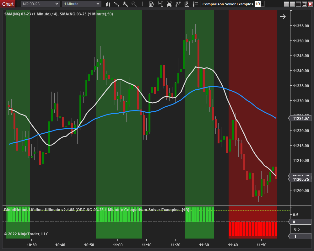
The chart below shows a Long output when the SMA 14 is 5pts or more above[>] the SMA 50, and a Short output when the SMA 14 is 5pts or more below[<] the SMA 50. In the two areas where there is no output, the SMA's are within 5pts of each other.
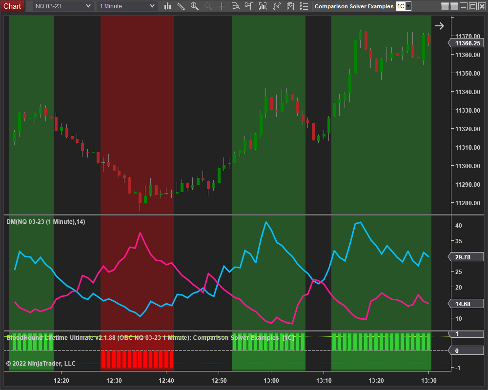
Example 1C: The Basics Using A Multi-Output Indicator
This demonstrates using the DM indicator with multiple plots. The Fixed rule is used to identify clear directional signals from the +DI & -DI plots. The Range rule is used to anticipate the beginning and ending of a trend direction by gradually increasing or decreasing the output value from 0.5 to 1 depending how far apart the DI plots are from each other, as seen in the chart below.
Input A & B Settings:
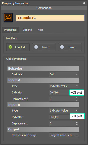
- Set Input A to DM » +DI plot.
- Set Input B to DM » -DI plot.
Rules window Settings:
Open the Rules window by clicking the ellipses button in section Output » Comparison Settings.
- Set up the Fixed rule as show below.
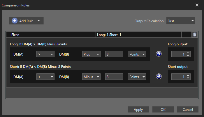
The chart below shows the choppy signals from the indicator are filtered out. Note, when the DI plots are within 2 points of each other there is no output.
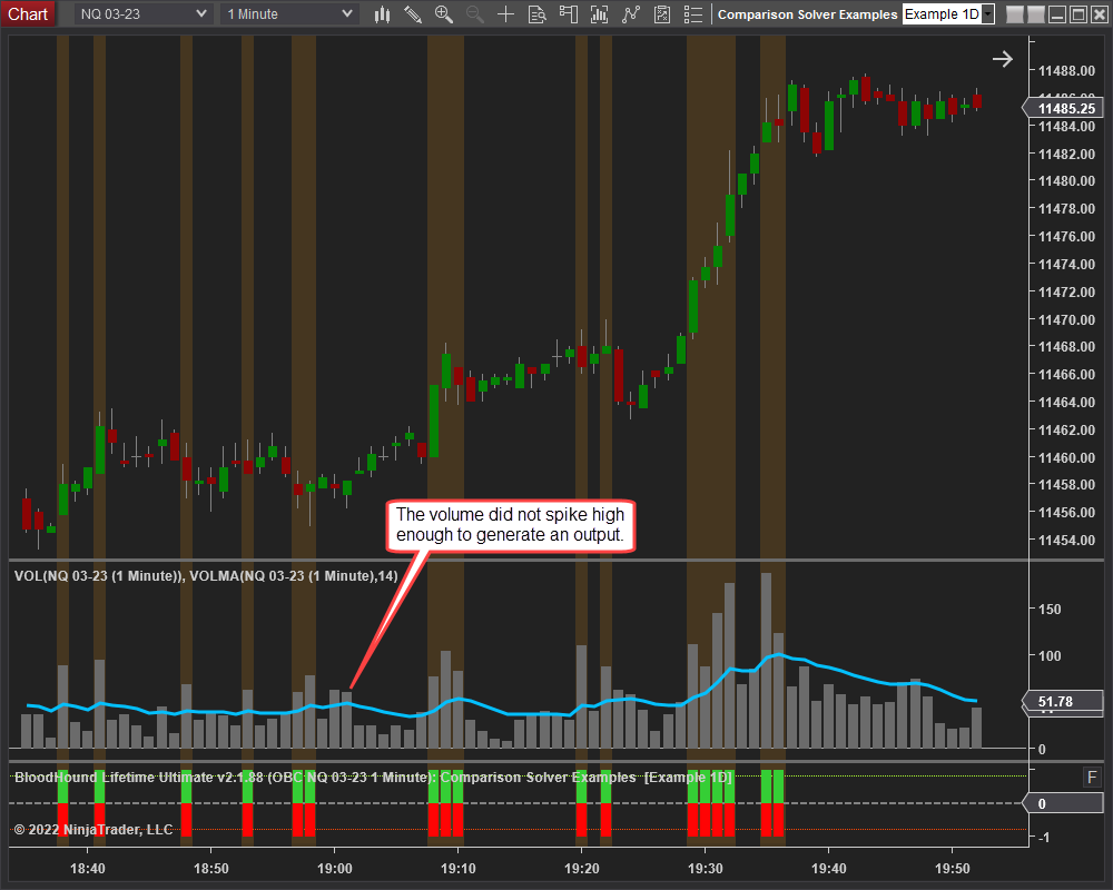
Example 1D: The Basics with Volume
This demonstrates using volume and a volume moving average with the Comparison solver. This example will generate a Long & Short output when the volume spikes above the volume moving average. Using the ATR as the Measurement Unit subjectively normalize the required amount for a volume spike, as the chart below shows.
Input A & B Settings:
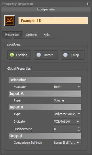
- Set Input A » Type to Volume.
- Set Input B to VOLMA 14.
Rules window Settings:
Open the Rules window by clicking the ellipses button in section Output » Comparison Settings.
- Set up the Fixed rule as show below.

The chart speaks for its self.
Example 2: Finding Higher Lows & Lower Highs
This demonstrates using the included Swing Highs & Lows indicator to identify higher lows (HL) and lower highs (LH). Input A is monitoring the indicator plots of the current bar. While, Input B is monitoring the indicator plots of the previous bar by setting the Displacement to 1. When the current bar's plot value differs from the previous bar's plot value the Comparison solver will detect that.
Input A & B Settings:
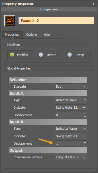
- Set Input A to the Swing Highs & Lows indicator as shown below.
- Set Input B to the Swing Highs & Lows indicator as shown below.
- Set Input B » Displacement to 1.
Swing Highs & Lows Properties and Plots
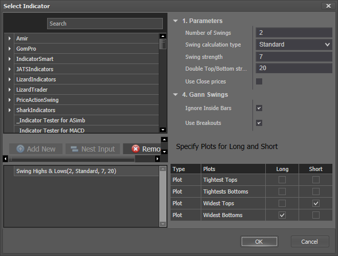
- Change the Swing Highs & Lows » Number of Swings property as shown.
- Select the same plots for Input A & B.
Rules window Settings:
No changes are needed to the Rules window.
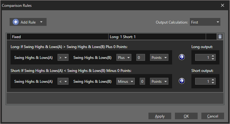
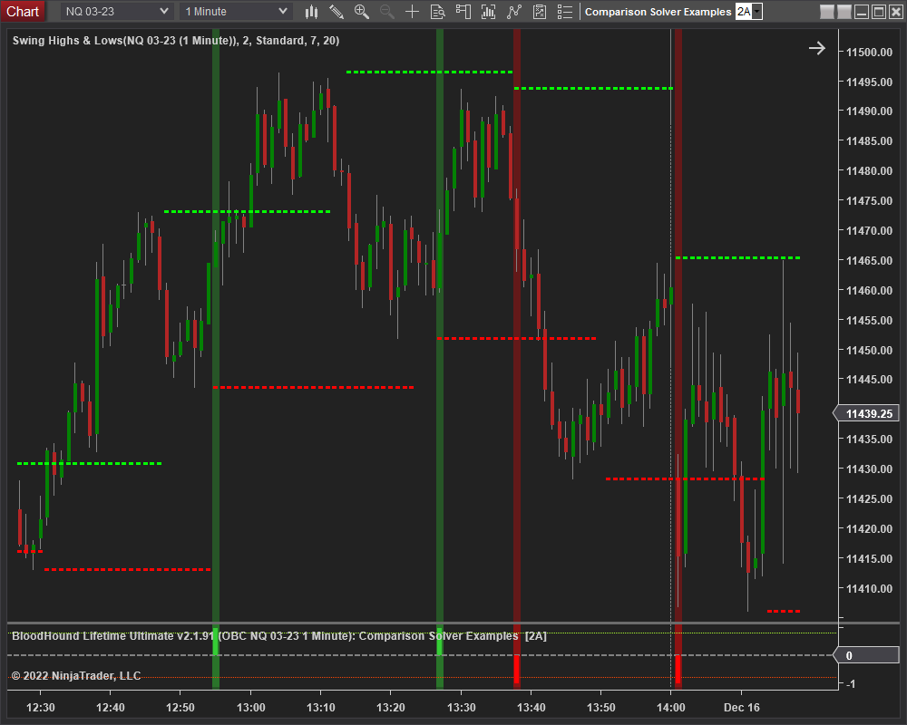
When the Widest Bottom (red hash) plot steps higher, a HL, a Long output is generated. When the Widest Top (green hash) plot steps lower, a LH, a Short output is generated.
BloodHound v1
Indicator Comparison Solver
Parameters
Input A
Difference (A-B)
Input B
Long Output
Short Output
Sets the solver’s Short output values as described in Long Output settings above.
Video Tutorial
This video is from our weekly Workshop on May 29th, 2015.
For more benefit please watch in full screen mode, as this video is recorded in HD.
Example: Show Long Signals Only When Price is Above an EMA (2 minutes)
Examples
Example 1A: The Basics
This demonstrates the basic function of Indicator Comparison solver with the use of a EMA 50 and the Closing price. This Solver will be used to determine if the Closing price is above or below the EMA 50.
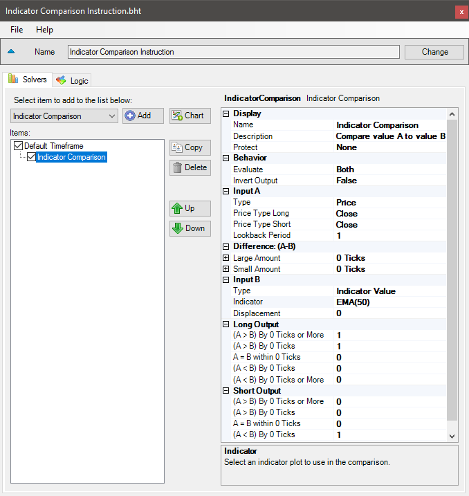
- Add the Indicator Comparison solver
- Set Input A Type to Price
- Set Input B to EMA 50
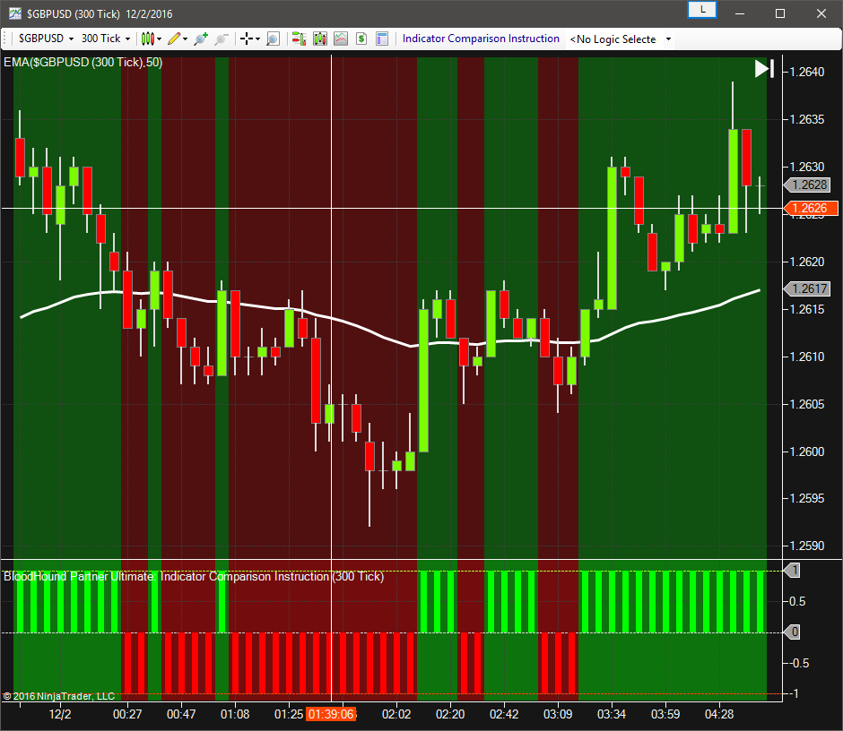
The chart below shows a Long signal when the Closing price is above the EMA 50, and a Short signal when the Closing price is below the EMA 50.
Example 1B: The Basics & A Little More
This demonstrates the use of Large Amount & Small Amount properties of the Solver with the same set up as above. This example sets the Solver to allow price to break through the EMA Support/Resistance line by 2 ticks and still provide a signal in the same direction with other indicator. As price moves from 2 ticks to 5 ticks away the output is reduced.
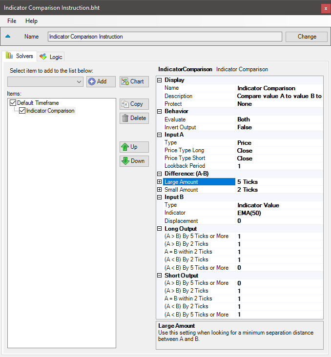
- Add the Indicator Comparison solver
- Set Input A Type to Price, and Input B to EMA 50
- Set Large Amount to 5 Ticks
- Set Small Amount to 2 Ticks
- Set Long Output values as shown
- Set Short Output values a shown
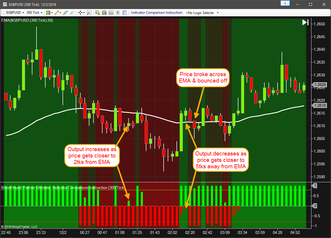
The chart below shows a Long & Short signal when the Closing price is within 2 ticks of the EMA. This is because Long Output (A < B) By Small Amount is set to 1, and Short Output (A > B) By Small Amount is set to 1 which causes a signal to occur even if the Closing price breaks the EMA, allowing for a more organic system.
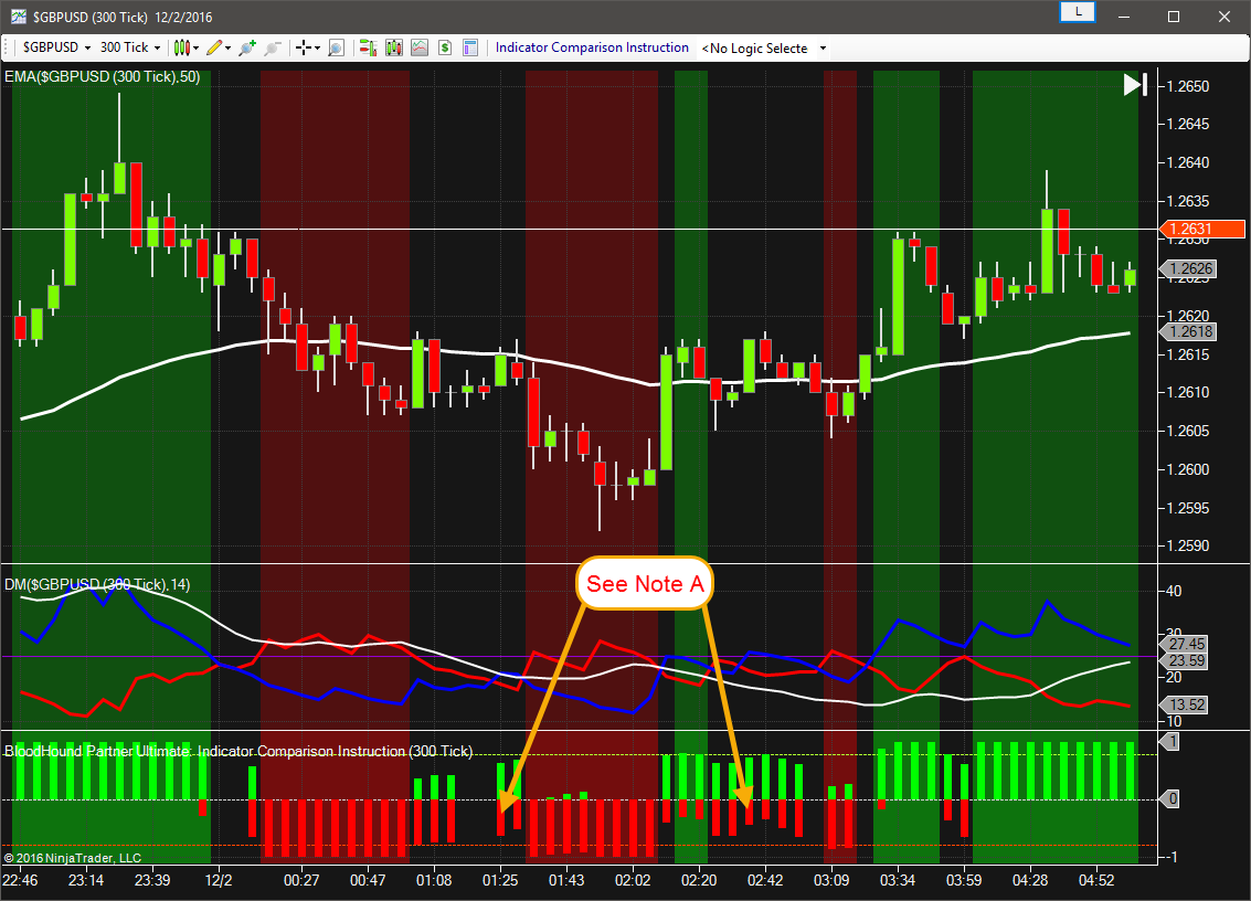
Example 1C: The Basics Using A Multi-Output Indicator
This demonstrates using the DM indicator with multiple plots. The Large Amount property is used to filter out unclear & choppy signals from the +DI & -DI plots. The Small Amount property is used to anticipate a reversal in signal direction by providing a 0.7 output value set in Long Output (A < B) By Small Amount and Short Output (A > B) By Small Amount.
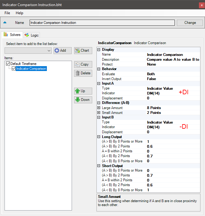
- Add the Indicator Comparison solver
- Set Input A to DM » +DI plot
- Set Input B to DM » -DI plot
- Set Large Amount to 8 Points
- Set Small Amount to 2 Points
- Set Long Output values as shown
- Set Short Output values a shown
The chart below shows the choppy signals from the indicator were filtered out. Note A: When the +DI & -DI are within 2 points of each other an output in the opposite direction is given.
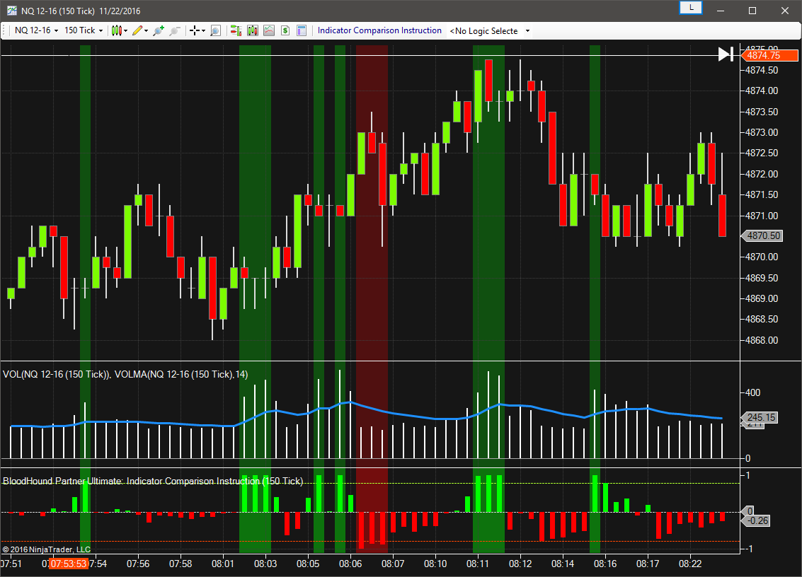
Example 1D: The Basics with Volume
This demonstrates using volume and a volume moving average with the Indicator Comparison solver. This example will generate a Long signal when volume spikes past the Large Amount, and generate a Short signal when volume drops below the Large Amount. The ATR is used in the Difference section to help normalize the volume’s volatility.
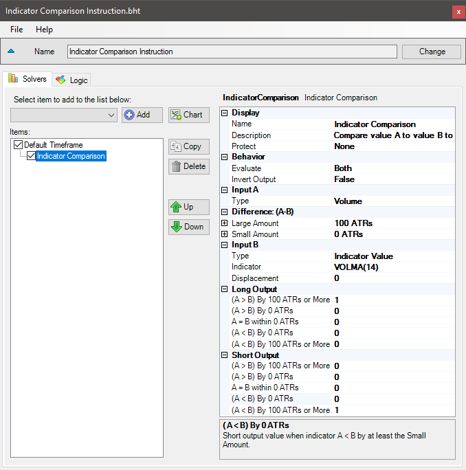
- Add the Indicator Comparison solver
- Set Input A Type to Volume
- Set Input B to VOLMA 14
- Set Large Amount to 100 ATRs
- Set Small Amount to 0 ATRs
- Set Long Output (A > B) By Small Amount to 0
- Set Short Output (A < B) By Small Amount to 0
The chart speaks for its self.
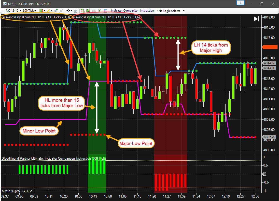
Example 2: Finding Higher Lows & Lower Highs
This demonstrates using the built in Swing indicator of different Swing Sensitivity with the Indicator Comparison solver. Indicator A is configured for minor swings. Indicator B is configured for major swings. The Solver will look for higher low points of 15 ticks or greater for a Long signal, and lower high points of more than 15 ticks for a Short signal.
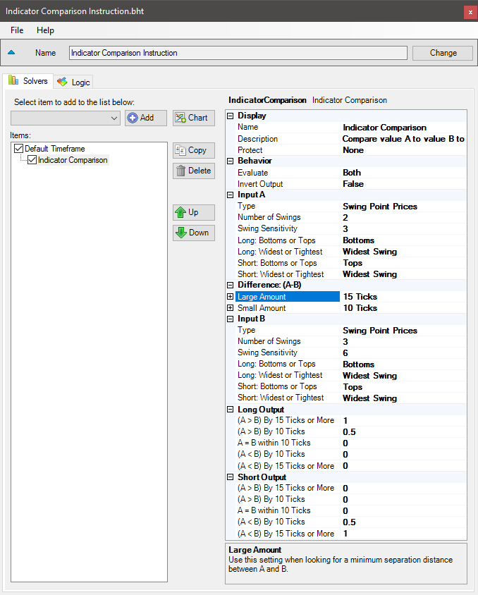
- Add the Indicator Comparison solver
- Set Input A Type to Swings
- Set Input A values as show
- Set Input B Type to Swings
- Set Input B values as show
- Set Large Amount to 15 Ticks
- Set Small Amount to 10 Ticks
- Set Long Output (A > B) By Small Amount to 0.5
- Set Short Output (A < B) By Small Amount to 0.5
Notice on the chart, the lower high was 13 ticks instead of 15 ticks as set in Large Amount and a signal was given. This is because the Short Threshold is set to 0.8 (80%), the Small Amount is set to 10 ticks, and Short Output (A < B) By Small Amount is set to 0.5. At 10 ticks the output = 0.5. Small Amount to Large Amount is 5 ticks, so every tick = 0.1 in the output. Therefore 10 ticks = 0.5, next 3 ticks = 0.3. Result is 0.5 + 0.3 = 0.8