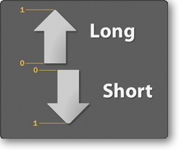
BloodHound works using fuzzy logic principles to calculate it’s intermediate and final output values (known as confidence values).  Confidence values are a decimal number ranging from 0 to 1.0 that represents a percentage of confidence (0% to 100%).  The lower the number, the less favorable it is, and the higher the number (approaching 1.0) the more favorable the condition is.  At each stage of calculating an output value for a particular bar (or tick) BloodHound maintains a separate value for the Long side and the Short side.  Thus, the Long and Short sides are always evaluated simultaneously, but separately.  Note: internally the short side is always calculated as a positive value even though the Short Confidence plot is displayed on the chart as a negative value (0 to –1).  The short side’s internal positive value is converted to a negative value for visual purposes when it is plotted to the chart.

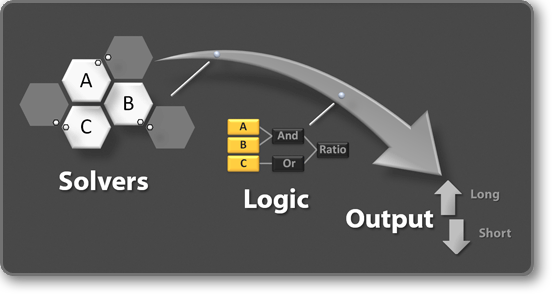
There are two components at play in every BloodHound configuration (called a BloodHound template, which we will be abbreviating BHT for short).  A BHT contains two types of objects:confidence solvers (solvers for short) and logic templates.  Each BHT can have multiple Solvers, and multiple logic templates defined.  Each of the two components play an important role in configuring BloodHound to arrive at a final output.

You can think of the BHT as the main parent document that encompasses all your settings.  BHT’s are saved and loaded in the form an XML file, thus remembering all your configuration settings for a particular strategy you’re working on.  The default location for these files are in your NinjaTrader documents directory under:

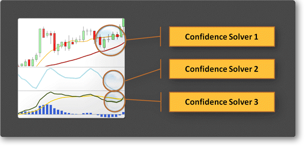
The first stage of every BloodHound calculation involves gathering data from the solvers defined in the BHT.  Solvers are the raw inputs derived directly from observations on the chart, price bar action, swing trends, support and resistance etc.  There are also solvers that can be configured to look at a particular indicator values, compare indicator values from another or even examine the sloping behavior of an indicator.  A list of these solvers is found here.

Your end goal may be to identify desired trade signals, or to alert you to an impending trade setup.  Either way, it all starts with the solvers that you add to your BHT.  The solver’s raw output data is then processed by your logic template which you define separately.  The combination of raw data generated by your solvers together with your logic configuration produces BloodHound’s final output.

Each solver looks at one particular aspect or feature of your chart, and so to examine multiple aspects of your chart, you would employ multiple solvers, each designated to look at different areas of interest.  You can commission as many confidence solvers as you like in your BHT, but remember the more solvers you have, the more work BloodHound has to do to calculate your result.  Generally speaking it is good practice to use only the solvers that are necessary to produce your end result, and remove solvers that aren’t contributing anything to the final calculation.

Solvers produce a confidence value between 0 to 1.0 (0% to 100% confidence) for both the long and short sides simultaneously for every bar (or tick).  You can think of solvers as a way to interpret what you’re seeing on your chart and translating that into a grading score between 0 and 1.0 for each side.  For example, let’s say you’re interested in the slope of a particular indicator.  Part of your trading system dictates that a positive slope is good for long trades, and negative slope is good for short trades.  To represent this aspect of your trading system, you would add an Indicator Slope Solver to your BHT, and configure it to give you a 1.0 on the long side and 0 on the short side when the slope is positive, and a 1.0 on the short side and 0 on the long side when the slope is negative (this is actually the Indicator Slope Solver’s default behavior already).  You would then add other solvers to the BHT to represent the other aspects of your trading system.

The Logic template system is where the real power and flexibility of BloodHound exists, and is considered the second essential component to a BHT.  Logic templates describe how to compute the final results from your input data.  This is achieved by manipulating a node diagram much like an electronic logic board.  With logic you can manipulate the raw output produced from solvers and create constructs that produce outputs to match your specific goals.  The logic template is flexible enough to allow you to chain outputs to inputs to outputs and so fourth, allowing you to design a logical system with any degree of complexity.

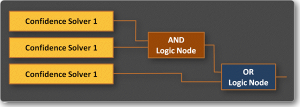
Solver nodes are added to these logic templates and are connected to logic nodes (such as the AND, OR,XOR, Ratio and Additive nodes).  These logic nodes combine and manipulate the outputs from the solver nodes to achieve a desired logical calculation.  For example, suppose you had two solver nodes, one that measured if the slope of an indicator was favorable in a given direction, and the other measured whether the current price was far enough away from a support/resistance zone to take a trade.  Your trading system rules dictates that both conditions must be “good” in order to take a trade (by default, good would be a value equal to or greater than 0.8).  Thus you would connect both of these solvers to the logic template, and then connect them together with an AND logic node.  The result would guarantee that both solvers had to be producing favorable values (above 0.8) in order to result in a valid trade signal.

In your BHT, you can have multiple logic templates defined.  Generally you select one logic template to be active at any given time (although a NinjaTrader strategy may incorporate the values of several logic templates simultaneously).  The active logic template will paint the chart with the resulting output signals in the form of red and green stripes (called racing stripes).  You may switch the active logic template at any given time while running BloodHound as an indicator by accessing the drop down at the top of you NinjaTrader chart.

You can pan around the Logic Board work area (dark green area) by using the middle mouse button (typically the wheel on your mouse).  By click-dragging with the middle mouse button you can pan around the workspace.  Alternatively, you can click the hand icon to toggle panning mode on or off.  To zoom in and out, use the mouse wheel.

To start working with the Logic template workspace, first navigate to the Logic tab.  Before you start, you may need to add a new Logic template by clicking the New Logic button.  You’ll notice three important menus: Solver nodes, Function nodes, and Logic nodes.  Each of these menus list the various types of nodes that can be added to the logic workspace area below.

You can move nodes around the workspace as you wish by click dragging them individually, or selecting several of them by first clicking on an empty spot and dragging the selection box over the nodes you want to select.  Notice that when you select a single node, the right hand side panel updates with information on that node.

Solvers that you have added earlier will each appear in the Solver node’s panel.  You will notice that when you add a node to the logic board, it will have a single green dot on the right side.  This dot is the node’s output connector point.

There are also a number of logic nodes: AND, OR, XOR, Ratio, and Additive.  These can be added in a similar manner.  You will also notice after adding any of these nodes that there is an Input connector and an Output connector.  Generally speaking, you create meaningful logic by connecting the output of Solvers to the input of Logic nodes.  To do this, simply move the mouse over to the node you want to wire data from (for instance a Solver node) and then click drag the leader to the node you want to wire data to (the destination node, typically a logic node).

Finally, you will also notice a special node already present on the workspace labelled ‘Result’.  This is where you connect your final logic output to.  The Result node plots whatever output is connected to it to the chart.

Connections/leaders between nodes can be deleted by mousing over to a connection line.  Then a red X icon will appear.  Clicking this red X deletes the connection.  Similarly nodes themselves can be deleted by clicking the red X button in the top right corner of the node, or by hitting the Delete key on the keyboard when the node is selected.